
Sediment Budget for Stanford Lands
Estimating annual erosion caused by the rain on a site is important for assessing the impact of human activities on the landscape, such as crop management and urban area expansion.
In this project, I used a simple widely used model in pedology known as the Revised Universal Soil Loss Equation (RUSLE) to estimate the amount of sediment eroded in Stanford lands for the year of 2017.
It is important to keep in mind that the RUSLE model was developed by USDA with data from the east coast. Applying it to the west coast requires an extra caution, here it only provides a rough estimate of erosion.
The soil loss equation is as simple as:
\[A = RKLSCP\]with
- \(A\) = soil loss (tons per acre)
- \(R\) = rainfall erositivity index
- \(K\) = soil erodibility index
- \(L\) = hillslope-length factor
- \(S\) = hillslope-gradient factor
- \(C\) = cropping-management factor
- \(P\) = erosion-control practice factor
Below I go over the process of estimating each of these parameters with data from rainfall gauges near Stanford lands and satellite images.
Erositivity index (\(R\))
This index translates the potential of the rain in eroding the soil (mostly interill) and depends on rainfall observations or rain forecasts for the year. Since we don’t have a good forecast model, we will use historical data from rainfall gauges installed in the Santa Clara County.
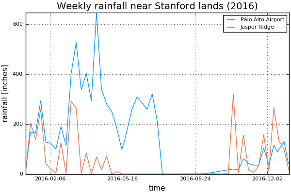
I used rainfall measurements from a tipping bucket rain gauge installed in Palo Alto airport. The data is available online in the website of the Department of Water Resources in California. I also used rainfall measurements from the Jasper Ridge Preserve as the second closest rainfall station.
For 2016, the data looks like the following:
The rainfall intensity in inch per hour can be approximated by dividing the amount of rain over the number of hours in the timescale (e.g. days, weeks):
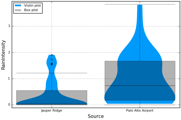
We observe that the intensity in Palo Alto Airport is statistically higher than the one in Jasper Ridge. To be conservative, we base our estimate of erositivity on the Airport data.
From the rainfall intensity \(I\) in inches per hour, we can estimate the kinetic energy \(E = 916 + 331 \log_{10} I\) in foot-tons per acre per inch of rainfall. I consider a few storms, shaded in green in the rainfall intensity plot below:
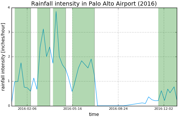
For each storm I record the maximum 30-minute rainfall intensity, and estimate the kinetic energy by means of numerical integration. The erositivity index is then computed by summing up the contribution of each storm.
The estimate is \(R \approx 43.79\).
Soil erodibility index (\(K\))
This index translates the tendency of a soil to be detached from the land surface during the rain. Wischmeier and Smith 1965 obtained \(K\) values for different soils via direct field measurements. An updated \(K\) factor map by esri is available in ArcGIS. The estimates do not vary much on the site and I just used the average value as an approximation from the screenshots below:
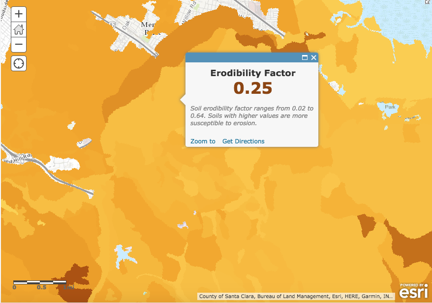
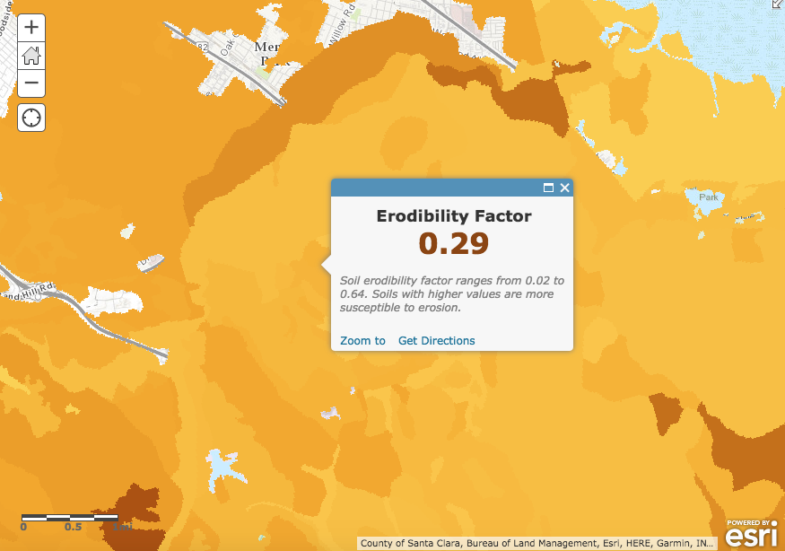
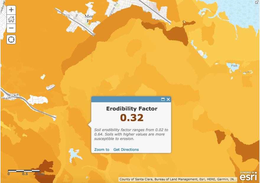
\(K = (0.25 + 0.29 + 0.32)/3 \approx 0.29\).
Hillslope length-gradient factor (\(LS\))
For the hillslope factors I used the USGS national elevation dataset 1/3 arc-second. I processed the elevation map in Google Earth Engine and computed the slope near Stanford lands (delineated in red):
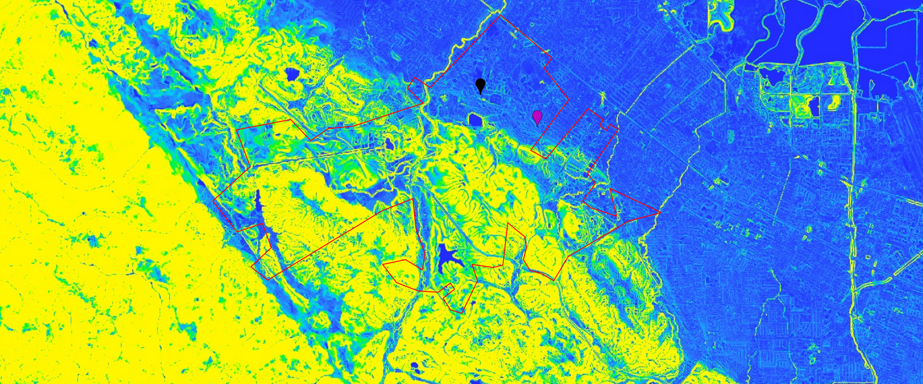
To give a sense of scale, I pin pointed the Green Earth Sciences building in black and the Rains Graduate Housing in the eastern side of the campus.
I then plot the histogram of slopes inside of the area delinated in red for estimating the \(LS\) factors:
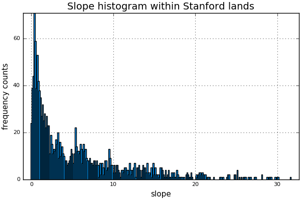
We observe that the land is quite flat, with a few exceptions near the mountain area. I estimate the median slope and use it instead of a more detailed break up of the land into regions of different slope. This approximation is very rough but I consider it to be enough for the purposes of this project. The median slope is approximately \(3.356\).
I then estimated a few slope lengths within the lands by using the slope map above. I simply dropped markers in the map and computed the geodesic distance between them. Some of the values I obtained include \(282ft\), \(250ft\), and \(118ft\). I simplify the problem using an average slope length. The mean slope length is approximately \(216.6ft\).
Using the estimates for slope percentage and slope length, I entered in the calibrated RUSLE table and read the value for the LS factor:
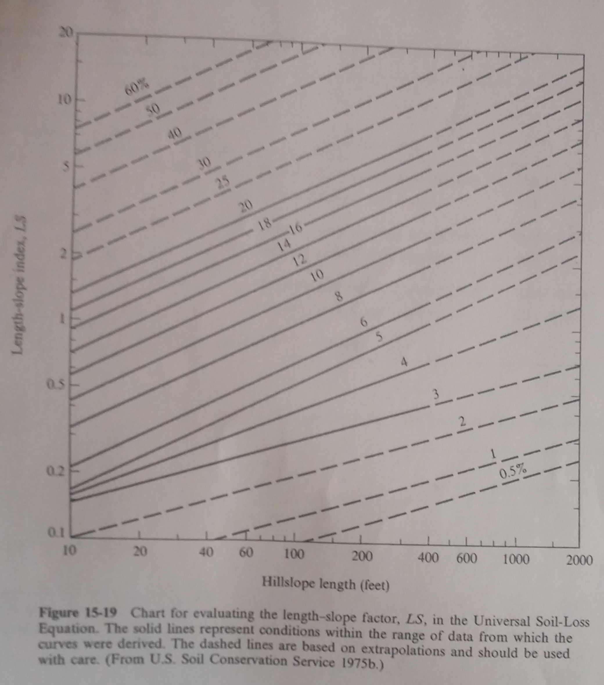
The estimate is \(LS \approx 0.4\).
Cropping-management factor (\(C\))
For the cropping-management factor I used the GLCF landsat tree cover continuous fields dataset. Similarly to the terrain slope, I plotted the histogram of vegetation height within Stanford lands:
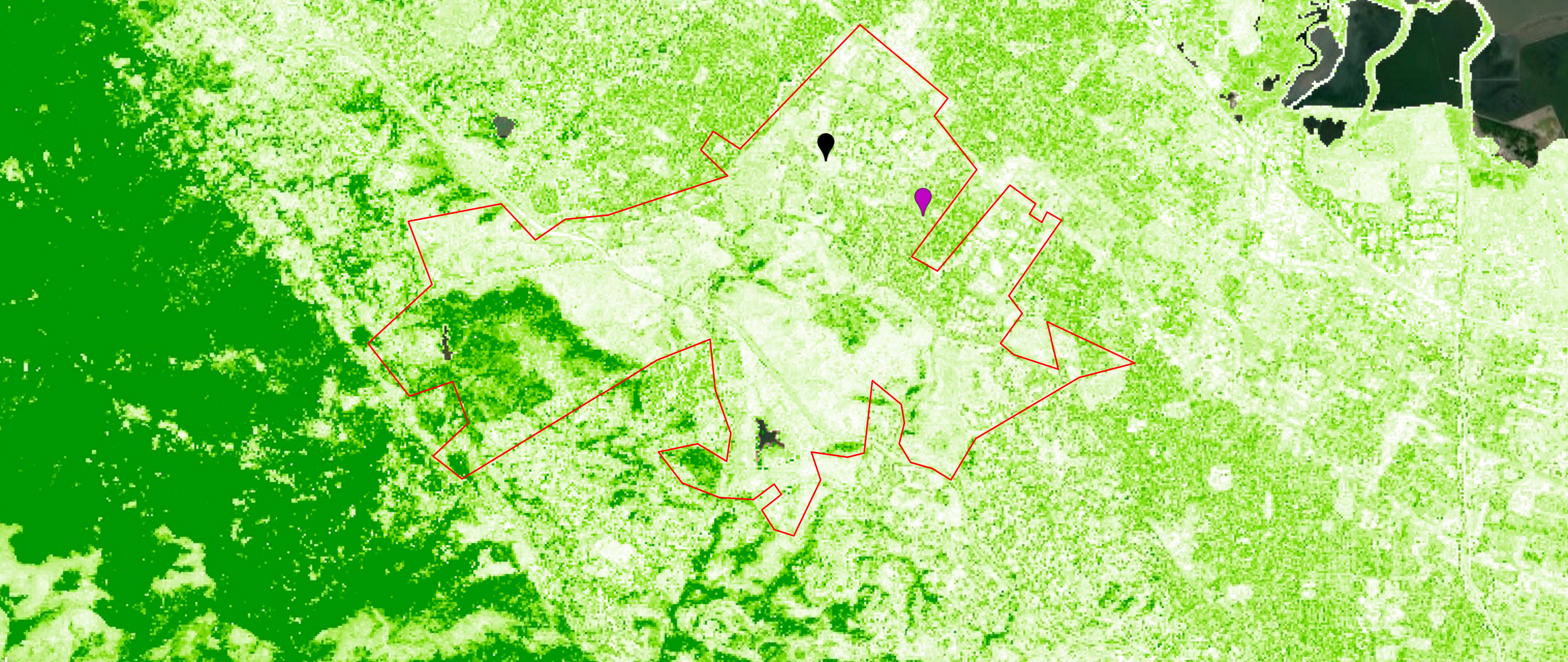
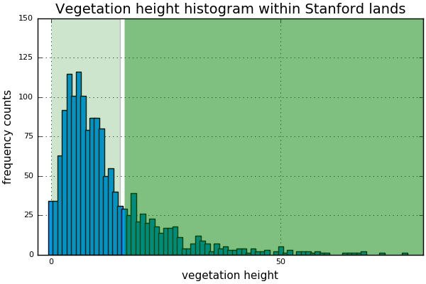
We observe that the vegetation on these lands is mostly grass camps in light green color in the map. A few canopy exist near the mountains and are represented in dark green. We estimate the percentage of canopy and ground cover by grass using the weights of the histogram. The canopy is responsible for approximately \(27\%\) of the area within Stanford lands whereas the rest is occupied by grass camps.
Using the RUSLE calibrated table, I enter “Tree but no appreciable low brush”, then canopy cover of approximately 25%, cover at surface is grass (G), and finally interpolate (linear interpolation) between the values associated with 60% and 80% grass cover.
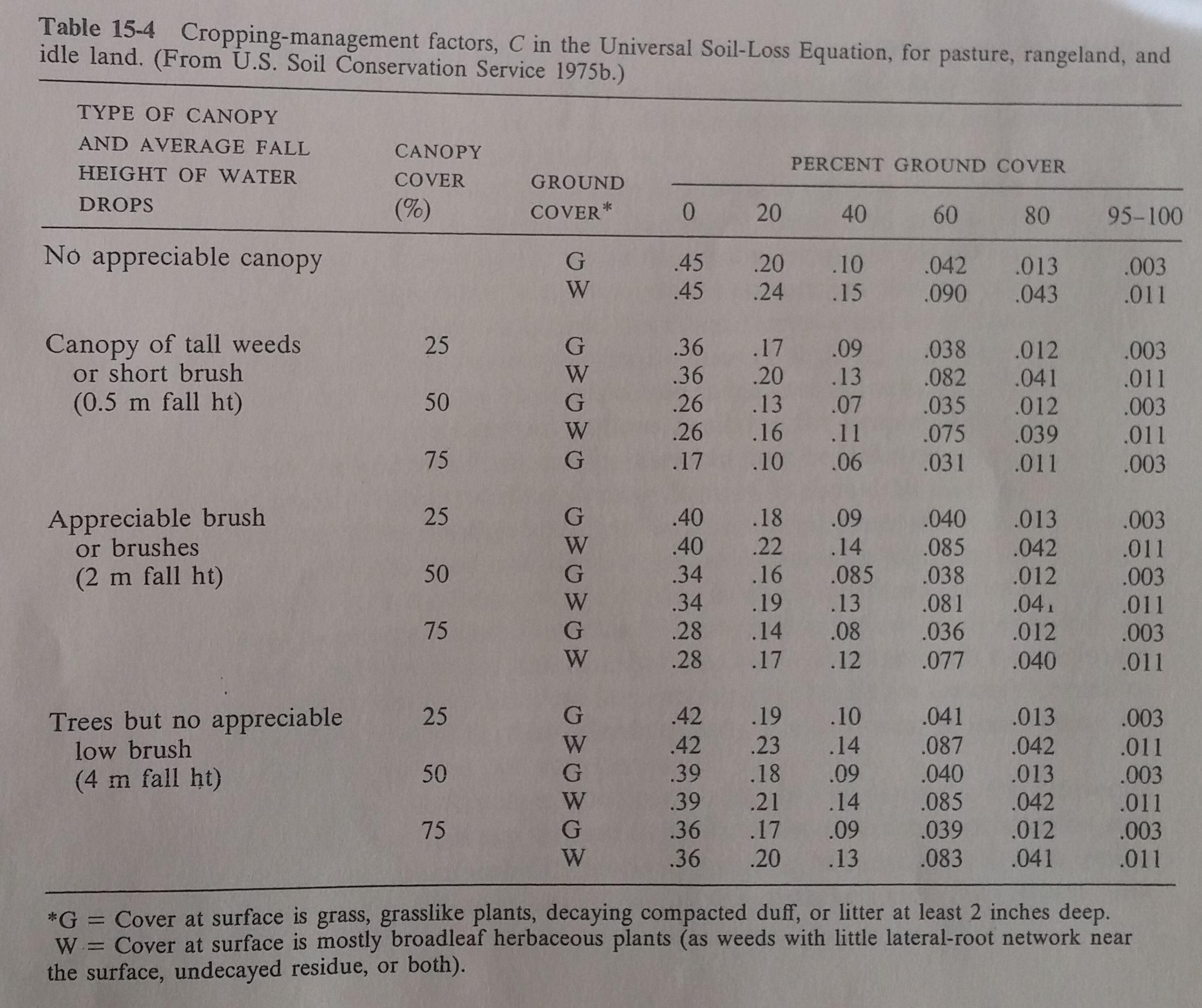
The estimate is \(C = (0.041 + 0.013) / 2 \approx 0.027\).
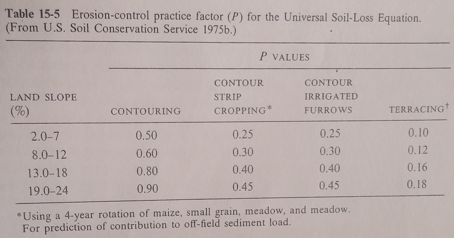
Erosion-control practice factor (\(P\))
Using the median slope computed in the previous steps, I enter in the RUSLE calibrated table with land slope between 2-7%. Since we don’t have any rotation on these lands (as far as I know), I assume the \(P = 1\), meaning no correction.
Annual sediment budget (\(A\))
Finally, having estimated all the factors in the RUSLE model, we can estimate the annual erosion as \(A = RKLSCP \approx 0.13\) tons per acre. Because Stanford lands have \(37km^2\) (or \(9142.9\) acres), this is about \(0.8\) inches of erosion on average per year.