Flipping coins in continuous time: The Poisson process

In this post, I would like to contrast two ways of thinking about a coin flip process—one of which is very intuitive and one of which can be very useful for certain applications. This insight is inspired on a stochastic modeling class by Ramesh Johari.

Discrete-time coin flip process

Suppose that I ask you to simulate a sequence of i.i.d. (independent and identically distributed) coin flips in a computer where the probability of flipping a coin and observing a head () is \(p\) and the probability of flipping a coin and observing a tail () is \(1-p\):

, , , , , , \(\cdots\),

There are at least two ways of doing this:

Solution A — popular solution

The most popular solution by far is to go to your favorite programming language (e.g. Julia ) and sample a sequence of \(Bernoulli(p)\):

using Distributions

p = .5  # probability of head
N = 100 # number of coin flips

coin_flips = rand(Bernoulli(p), N)
# 1, 0, 0, 0, 1, 1, ...

Solution B — not so popular solution

Think of a head (or \(1\)) as a successful coin flip. For example, you earn $1 whenever the head comes up and nothing otherwise. Keep track of the times when you had a successful outcome \(T_1,\; T_1+T_2,\; T_1+T_2+T_3,\; \ldots\)

Now is the trick. In a \(Bernoulli(p)\) coin flip process, the interarrival times \(T_n\) between successes are i.i.d. \(Geometric(p)\). Instead of simulating the coin flips directly, simulate the times at which a head will occur:

using Distributions

p = .5 # probability of head
N = 100 # number of coin flips

T = rand(Geometric(p), N)
head_times = cumsum(T+1)
head_times = head_times[head_times ≤ N]

# construct process in a single shot
coin_flips = zeros(N)
coin_flips[head_times] = 1
# 1, 0, 1, 1, 0, 0, ...

Why is solution B relevant?

In other words, why would you care about a solution that is more verbose and somewhat less intuitive?

Imagine that the probability of success \(p\) is extremely low. Would you like your computer spending hours generating tails (or \(0\)) before it can generate a head? For some applications, this is a critical question.

More than that, sometimes Solution A is not available…

Continuous-time coin flip process

The Poisson process is the equivalent of the coin flip process in continuous-time. Imagine that you divide real time \(T\) (a real number) into small intervals of equal lenght \(\delta\):

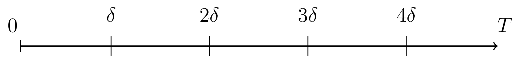
If a coin is to be flipped at each of these marks in the limit when \(\delta \to 0\), then Solution A is not available! There are uncountably many coin flips in the interval \([0,T)\).

However, simulating this process in a computer is possible with Solution B. For a Poisson process with success rate \(\lambda\), the interarrival times are i.i.d. \(Exponential(\lambda)\).